When I search for the word ‘consistent’ in Greene’s econometrics textbook, my pdf reader returns 523 matches! Likewise when I search for the word ‘bias’ or ‘efficiency’, my pdf reader returns 432 and 146 matches respectively. Clearly, they are extremely important concepts for learning econometrics.

Collectively, bias, efficiency and consistency represent three fundamental properties of estimators. These concepts come up everytime a researcher has to choose between the results of two different methods. In this blog post, I try to explain the principles behind these concepts intuitively using story-telling and simulations rather than relying on math. This might help readers understand the principles with more clarity and understand how it is used in mordern econometrics.

Female heights

Imagine for a moment you were God and you could observe the heights of all 1 million adult females on the face of planet Earth. And if you had to summarize the distribution of heights you would say that it had a mean of 5.2 and standard deviation of 0.2.

What would such a population look like?

set.seed(123)
population <- rnorm(10e5,5.2,0.2) 

data.frame(obs = population) %>%
  ggplot(aes(x = obs)) +
   geom_density(col = "black") 

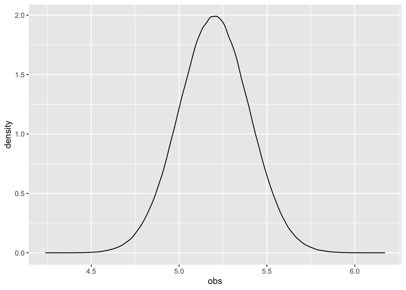
The distribution of heights for the entire population is bell-shaped with 5.2 in the middle.

Now, imagine that there was a researcher who wanted to figure out the most occurring height of adult female. And the researcher does not have access to any information about the population - neither can he see the picture above nor does he know the mean and standard deviation.

In statistical language, the most occurring height is the researcher’s parameter of interest. Let’s represent the sample parameter estimate by \(\theta\). The true value of this parameter is equal to 5.2. Let’s represent the true population parameter estimate by \(\theta^0\). The true value is unknown to the researcher because he can never have access to the heights of entire female population. Instead, he only has a tiny sample of 50 adults from this population.

research_sample <- sample(population,50)

data.frame(obs = research_sample) %>%
  ggplot(aes(x = research_sample)) +
   geom_density(col = "black") 

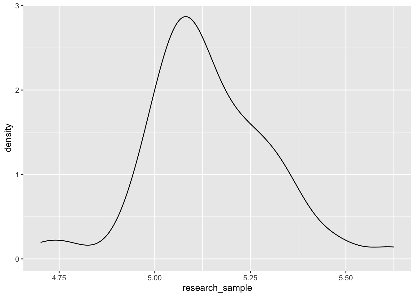
The graph on the right is what the sample distribution looks like. The distribution looks similar to the actual picture but kind of distorted.

He wants use this tiny sample to estimate the most occurring female height of the entire population. In order to estimate his parameter of interest he needs an estimator. An estimator is essentially a function that spits out an estimate (of most occurring female height in this case) when it is fed data from the sample.

Listen to the rumors

There are two separate rumors about how the heights of adult females might be distributed. One set rumors say that the distribution of adult female heights is bell shaped. That means the most occurring value should be closer to the center of the distribution. The other set of rumors say that the distribution of adult females is skewed. This means that the most occurring value of the distribution would be closer to minimum of the distribution. The researcher does not know which set of rumors to believe.

So he creates two estimators - estimator1 and estimator2. The first one attempts to find the centermost value in a sample - he finds the minimum of the second quartile and the maximum of the third quartile and divides the two numbers by 2.

estimator1 <- function(x){
  ( min(x[x > quantile(x,c(0.25,0.75))[1]]) + 
    max(x[x < quantile(x,c(0.25,0.75))[2]]) ) / 2
}

The second one attempts to find the minimum value in a sample - he finds the minimum in the first decile.

estimator2 <- function(x){
  min(x[x < quantile(x,c(0.1,0.9))[1]])
}

Using these estimators lets check the estimate of most occurring height ($\theta$) given the research sample -

estimator1(research_sample)

## [1] 5.140005

estimator2(research_sample)

## [1] 4.702334

Looks like the estimate from estimator1 is much closer to the truth compared to estimator2. But, of course the researcher does not know this.

Now that we have estimates from two different estimators, the real question is which estimator should the researcher pick? Is one better or superior than the other? To answer this question one needs to understand the characteristics of estimators and then use them to differentiate between a superior and inferior estimator.

In general, the characteristics of estimators is a description of how estimators are expected to behave given a random sample. These characteristics can be categorized based on the sample size. For smaller or finite samples, superior estimators will have no bias and will be more efficient. For larger or infinite sample sizes, superior estimators will be consistent¹.

Bias

To say that an estimator is unbiased means that on average the estimator would produce estimates that is close to the truth².

What does this mean in the context of our current problem? It means that if you could repeatedly draw samples from the population of adult females and allow an unbiased estimator to estimate the parameter of interest on each of the samples, then the average of the estimates would be similar to the true estimate of height 5.2.

Let’s visually inspect if this is true for estimator1 and estimator2. Below I draw a sample of 50 observations 5000 times from our population. And then I estimate the most occurring height using the two estimators.

n_iterations <- 5000
e1_estimates <- c()
e2_estimates <- c()
for (i in 1:n_iterations){
  sample_50 <- sample(population,50)
  e1_estimates[i] <- estimator1(sample_50)
  e2_estimates[i] <- estimator2(sample_50)
}

Below, I create a histogram of the estimates produced by the two estimators on each of the 5000 samples of 50 observations.

data.frame(estimates = c(e1_estimates,e2_estimates),
           draws = rep(c(1:5000),2),
           estimator = rep(c("estimator1","estimator2"),each = 5000)) %>%
  ggplot(aes(x = estimates)) +
   geom_density() +
   facet_wrap(~estimator,scales = "free") +
   geom_vline(xintercept = mean(population), col = "blue", lty = 2) 

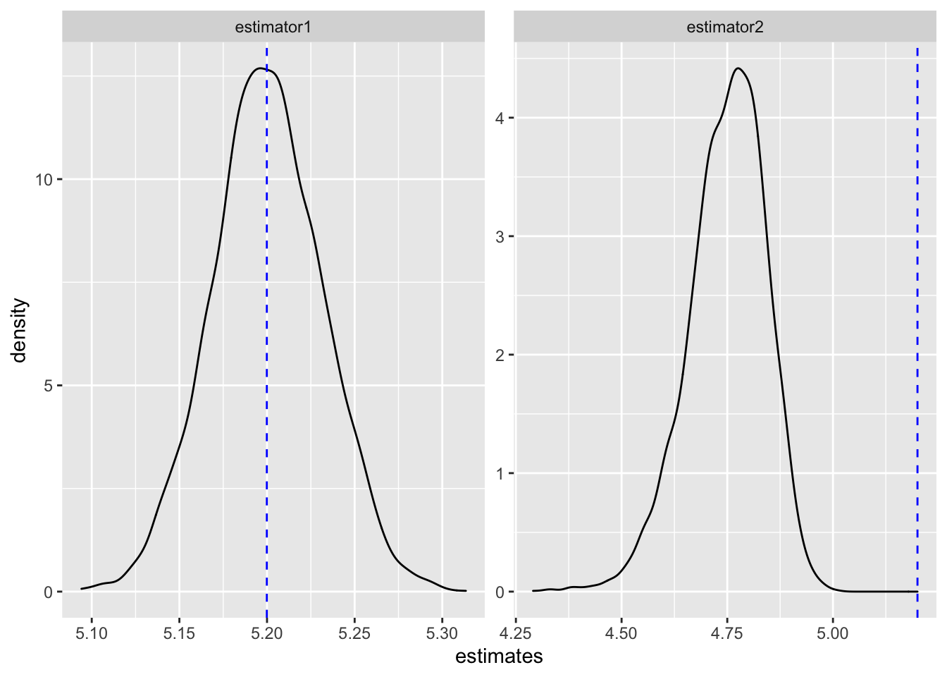
We can immediately tell which estimator performed better. The estimates from estimator1 was sometimes more than 5.2 and sometimes less than 5.2 but on average it estimated the correct value of 5.2 most of the time. This isn’t the story for estimator2. It has incorrectly estimated the true value of 5.2 for most of its samples. And so we say estimator1 is an unbiased estimator of most occurring female heights.

But, being unbiased is not always sufficient in deciding the superiority of an estimator. For example, if two estimators are both unbiased is there a way to break the tie and pick an estimator that is even better?

Efficiency

Realize that statistical inference isn’t always about getting an estimate. It is also about expressing uncertainty about that estimate³. This is the motivation behind the concept efficiency - you may have two estimators that give you the right estimates on average, but can one estimator be less uncertain than the other?

What does this mean in the context of our problem? It means that if you could repeatedly draw samples from the population of adult females and allow the efficient estimator to estimate the parameter of interest on each of the samples, then the standard deviation of the estimates would be small and tightly packed around the value of 5.2⁴.

To visually grasp the idea of efficiency we need a third estimator estimator3 which is as good as estimator1. Based on personal experience, the researcher somehow feels that the first rumor is true. If that is the case, then the most occurring height can also be approximated by the mean of a normal distribution. Accordingly, he models the sample heights as independent identically observations coming from a normal distribution. Then he finds the maximum likelihood estimate of the mean given the sample data.

estimator3 <- function(x){
  thet <- maxlogL(x = x, dist = "dnorm",
                  link = list(over = c("mean","sd"),
                  fun = c("log_link","log_link")))
  unname(thet$fit$par[1])
}

Now let’s visually inspect the efficiency of un estimator1 and estimator2. I draw 5000 samples of 50 observations and estimate the most occurring height using estimator1 and estimator3. Below, I compare the estimates from these two estimators.

n_iterations <- 5000
e1_estimates <- c()
e3_estimates <- c()
for (i in 1:n_iterations){
  sample_50 <- sample(population,50)
  e1_estimates[i] <- estimator1(sample_50)
  e3_estimates[i] <- estimator3(sample_50)
}

data.frame(estimates = c(e1_estimates,e3_estimates),
           draws = rep(c(1:5000),2),
           estimator = rep(c("estimator1","estimator3"),each = 5000)) %>%
  ggplot(aes(x = estimates)) +
   geom_density() +
   facet_wrap(~estimator,scales = "free") +
   geom_vline(xintercept = mean(population), col = "blue", lty = 2)

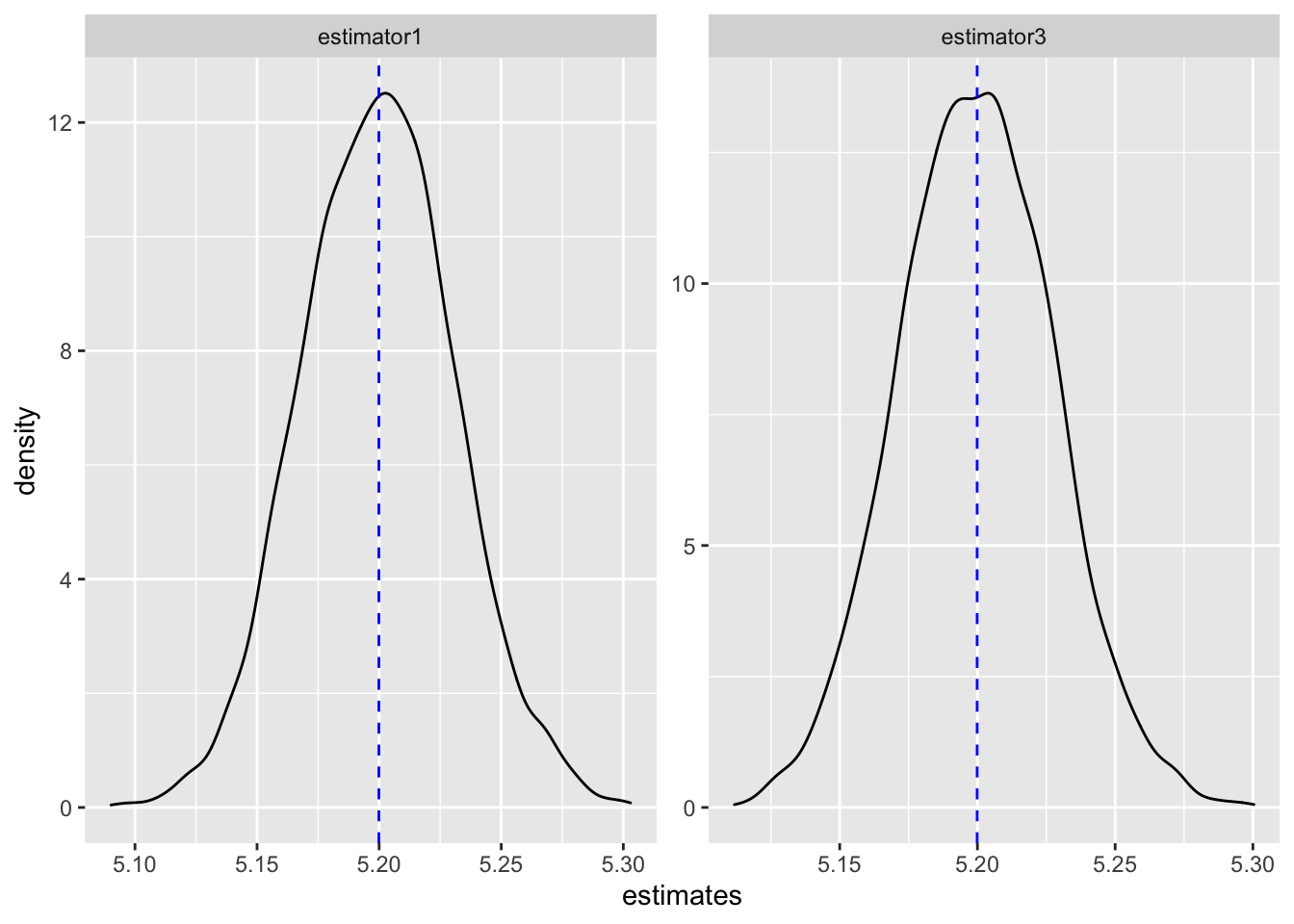
They are almost identical. They both appear to be unbiased when placed side by side. Now the researcher must choose between the two unbiased estimators. This is where efficiency can be used. Lets look at this plot slightly differently - lets overlay one histogram over the other instead of side by side.

data.frame(estimates = c(e1_estimates,e3_estimates),
           draws = rep(c(1:5000),2),
           estimator = rep(c("estimator1","estimator3"),each = 5000)) %>%
  ggplot(aes(x = estimates, fill = estimator, col = estimator)) +
   geom_density(alpha = 0.2) +
   geom_vline(xintercept = mean(population), col = "blue", lty = 2) +
   theme(legend.position = "top")

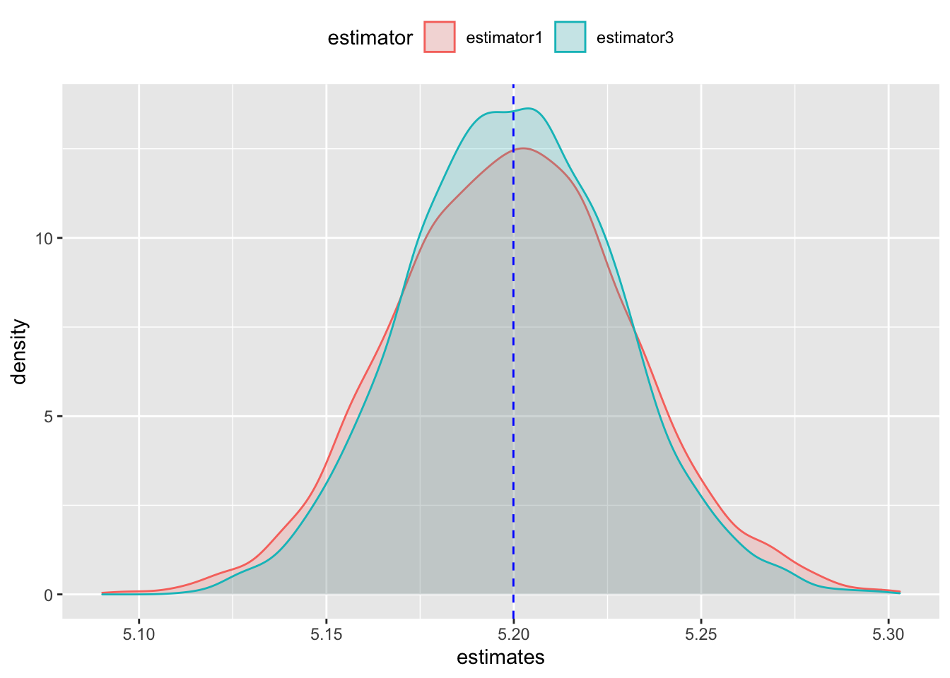
The subtle difference is now visible. The estimates produced by estimator3 is more concentrated around the true value of 5.2 compared to estimator1. In other words, the variance of the distribution of estimates from estimator3 is lower compared to estimator1⁵. We say estimator3 is more efficient than estimator1 because the former is less uncertain than the latter. It provides the researcher greater confidence in the sense that estimator3 is more likely to uncover the true value given a random sample.

To explain the concepts of biasedness and efficiency notice that I relied on repeated sampling from the actual population. This is not possible in practise. So, bias and effeciency of estimators are theoretical results are inspired by thought experiments where one imagines repeated sampling and uses known facts and theorems in statistical inference to arrive at a conclusion.

Consistency

The final important characteristic of an estimator is its consistency. An estimator is consistent if its estimate converges to the true value as the sample size gets infinitely large⁶. So unlike bias or efficiency, consistency involves changing sample size.

What does this mean in the context of our current problem? It means that if the researcher could repeated draw samples of increasing size from the population of adult females, the estimate from a consistent estimator would get closer and closer to 5.2.

Lets visually inspect the consistency for estimator1. I draw samples in increasing size of 50 repeated until the maximum sample size is 50000. Below I plot the estimates versus the sample size.

e1_estimates <- c()
samp_size <- seq(50,50000,50)
for (i in seq_along(samp_size)){
  e1_estimates[i] <- estimator1(sample(population,samp_size[i]))
}

ggplot(data.frame(n = samp_size,
                  estimates = e1_estimates),
       aes(x = n, y = e1_estimates))  +
  geom_point(size = 0.5) +
  geom_line() +
  geom_hline(yintercept = 5.2, col = "blue")

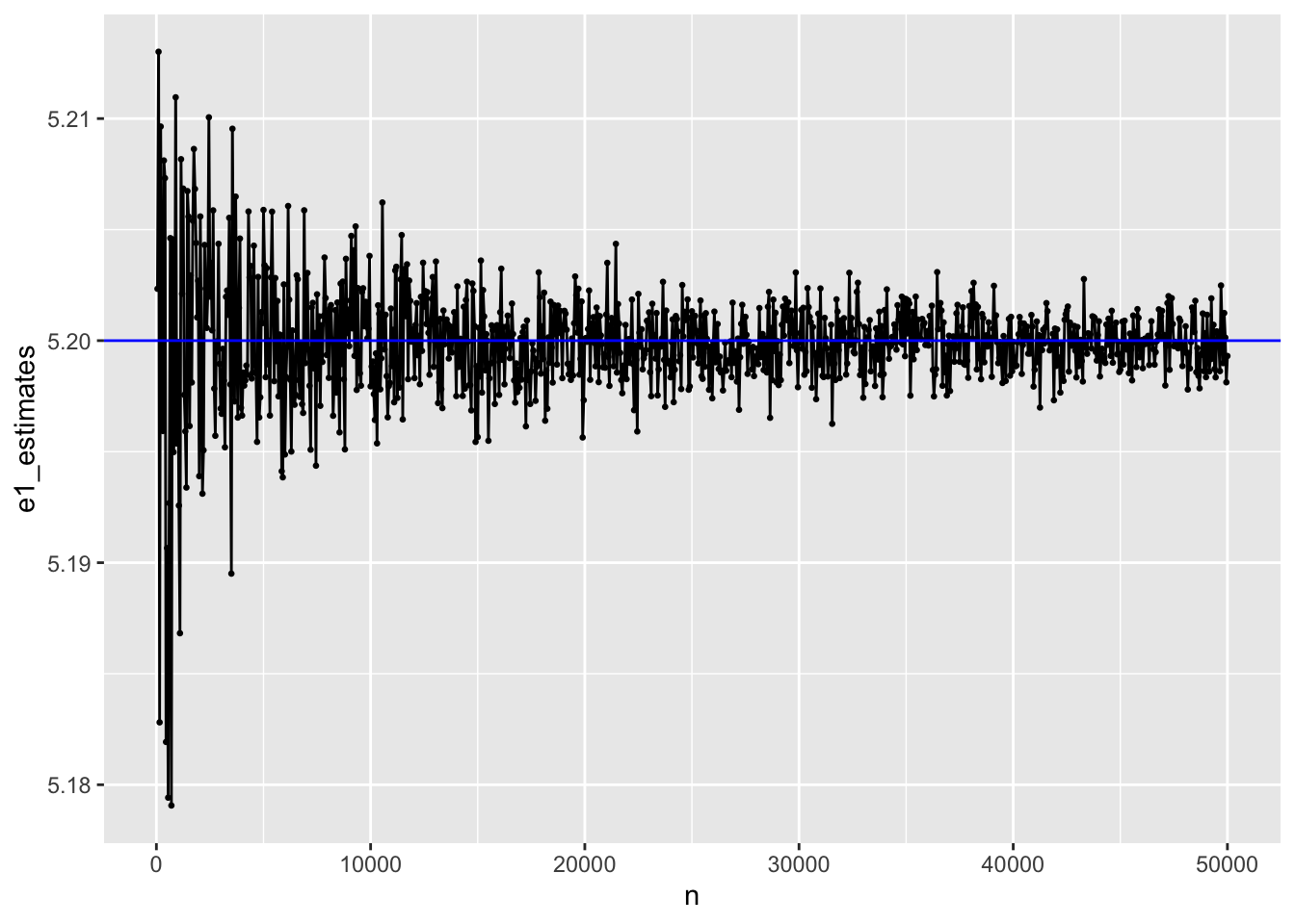
Indeeed, as the sample size gets bigger the estimate gets closer to the true value of 5.2. Notice how consistency encompases bias and efficiency⁷. As the sample size is increased, the estimated parameter gets closer to the actual value - estimator1 is unbiased for large sample sizes. As the sample size is increased the parameter values are less “wobly”. They seem to settle down and become concentrated around a point - estimator1 is efficient for large sample sizes.

I interpret the results in the graph in probabilistic terms to describe consistency more concretely. To do that first I measure the difference between the estimates produced by e1_estimator and the true value of 5.2.

difference <- e1_estimates - 5.2

Next, I check if the difference exceeds a small positive constant of 0.001 and count the number of times the difference has exceeded the positive constant.

threshold <- ifelse(difference > 1e-3,1,0)

Finally, I check the fraction of positive outcomes for various sample sizes in increasing order. The positive outcomes indicate the difference is more than the specified threshold.

# a helpful function to calculate the probability
get_prob <- function(l1,l2){
  l1 <- which(samp_size == l1)
  l2 <- which(samp_size == l2)
  vec <- threshold[l1:l2]
  table(vec)[2]/length(vec)
}

# Pr(theta - 5.2 > 0.01)
# sample sizes between 50 and 10,000
get_prob(50,10e3)

##    1 
## 0.42

# sample sizes between 10,000 and 30,000
get_prob(10e3,30e3)

##         1 
## 0.2418953

# sample sizes between 30,000 and 50,000
get_prob(30e3,50e3)

##         1 
## 0.1895262

You can see as the sample size gets larger the probability gets smaller and smaller. In other words, as \(n\) increases there is a greater chance that the estimated value would be similar to the true value. Can consistency be measured in practise? No. Similar to bias and efficiency, consistency is a theoretical concept.

Important facts

• In practise, we rather have an unbiased estimator than an efficient one
• If we have two unbiased estimators, we should ideally pick an efficient one.
• Consistency is a minimal requirement for an estimator. Because if an estimator is inconsistent, then we cannot be confident that it is good enough for inference even if we have a huge sample.

Approximating shapes

So far we were visually inspecting how the estimates from our estimators would look like. And that was possible only by repeatedly sampling from the population. This is not possible in reality. So, how can one infer about the shape of the distribution to get some sense of the uncertainties of the estimator?

Asymptotic normality comes to our rescue. It states that as sample size gets large, a sequence of random numbers will have a standard normal distribution. When asymptotic normality is true for a sequence of estimates coming from an estimator, it means that probabilities regarding these estimates can be approximated using standard normal probabilities. The central limit theorem (CLT) can also be used to make similar statements about a distribution of estimates. It states that the average of a sample when standardized will have asymptotic normality. So, if we took the average of estimates and standardized it, it would be normally distributed with mean 1 and standard deviation 0.

Lets inspect if this is true for estimator1. I do two things - I increase the sample size from 5 to 60 and for each sample size I repeat the process several times to get a distribution of values for each sample size.

n_iterations <- 1:100
samp_size <- seq(5,100,5)
e1_estimates <- matrix(NA,
                       nrow = length(n_iterations),
                       ncol = length(samp_size))

for (i in seq_along(n_iterations)){
  for (j in seq_along(samp_size)){
    e1_estimates[i,j] <- estimator1(sample(population,samp_size[j]))
  }
}

colnames(e1_estimates) <- samp_size

e1_estimates_dt <-
  as.data.frame(e1_estimates) %>%
  mutate(iter = 1:n()) %>%
  gather(key = sampl_size, value = estimate, -iter) %>%
  mutate(sampl_size2 = factor(sampl_size, levels = samp_size)) %>%
  group_by(sampl_size2) %>%
   mutate(z_estimate = (estimate - 5.2)/0.2) %>%
  ungroup()

ggplot(e1_estimates_dt,
       aes(x = z_estimate))  +
  geom_density() +
  facet_wrap(~sampl_size2)

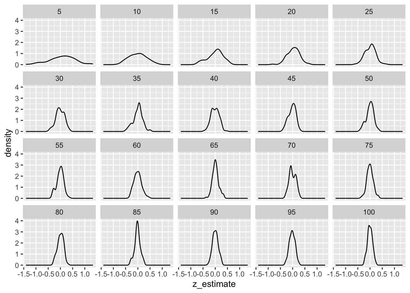
Indeed, as sample size increased the distribution of estimates starts to look more normal.