Sampling distributions of IVs

Using IVs to deal with omitted variable bias is very common in a variety of disciplines including marketing. In 2014, Peter Rossi published an excellent article in Marketing Science that highlights the major issues with the commonly used IV strategies in marketing. This article also provides an excellent overview of other IV topics such as (1) types of IV estimators and (2) the consequences of using weak or invalid IV.

He covers (2) in section 3.4 and 3.5 of this article where he provides an excellent illustration of the problem of weak and invalid IV from a sampling distribution perspective. Unfortunately, this section is also hard to understand for non-technical readers.

In this blog post, I try to elaborate on his main takeaways from section 3.4 and 3.5. I also use simulations to replicate the findings he presents in this section which might also help readers get more clarity when they read the actual article.

Two normals does not make a normal

Consider this linear regression model \(y = \beta x + \epsilon_y\). Now imagine we know that \(x\) is endogenous. The ordinary least squares (OLS) estimate of \(\beta\) that we get from this regression model, would be biased. To fix the issue, we estimate \(\beta\) using the two stage least square (2SLS) model. The 2SLS method involves finding an instrument \(z\) that explains the endogenous portions of \(x\) in a separate regression \(x = \gamma z + \epsilon_x\). We call this regression the first stage regression. We then use the predicted \(\hat{x}\) from this regression in the second stage regression \(y = \beta \hat{x} + \epsilon_y\). The \(\beta\) from this two stage process - \(\beta_{IV}\) - would be less biased compared to the OLS estimate of \(\beta\).¹

Matrix notation allows us to express \(\beta_{IV}\) more compactly in terms of \(z\), \(x\) and \(y\). You can algebraically show that

$$\beta_{IV} = \frac{z^Ty}{z^Tx}$$ Now, if \(z\), \(x\), and \(y\) are all normally distributed, the numerator and denominator in the expression above, are essentially two random variables that come from two normal distributions. In other words, \(\beta_{IV}\) is a ratio of two normal random variables.

$$\beta_{IV} = \frac{z^Ty}{z^Tx} = \frac{X_1 \sim N(\mu_1,\sigma_1)}{X_2 \sim N(\mu_2,\sigma_2)}$$

The question that Rossi asks in section 3.4 of his paper is this - does the distribution of the ratio of two normal random variables also look normal? He asks this question because understanding the distribution of the ratio of two normals would help understand the sampling distribution² of \(\beta_{IV}\).

So, below I generate two normal random variables - \(X_1\) coming from \(N(1,0.5)\) and \(X_2\) from \(N(1,0.2)\). Then I take their ratio and plot it.

set.seed(123)
ratio_normal <-
  data.frame(numerator = rnorm(10e4,1,0.2), #x1
             denominator = rnorm(10e4,1,0.2)) %>% #x2
  mutate(ratio_normal = numerator/denominator) %>%
  #zoom in a certain region
  filter(ratio_normal > -5 & ratio_normal < 5) 

ggplot(ratio_normal,aes(x = ratio_normal)) +
  geom_density(color = "black") +
  labs(x = "X")

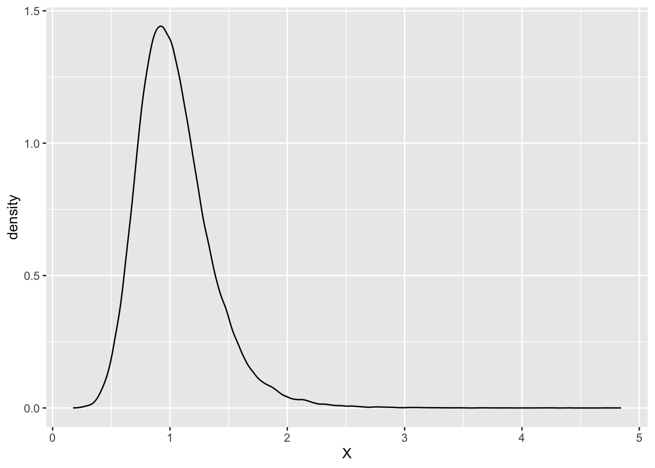
As we can see in this example, the distribution of the ratio of two normals does look normal. But, Rossi wanted to see how the above picture would change if we changed the distribution of the denominator. In particular, what would happen if we changed the denominator distribution so that it would have a larger standard deviation and a smaller mean.

Below I simulate the ratio of two normals again. But, this time once with \(X_2 \sim N(1,0.2)\) and then with \(X_2 ~ \sim N(0.1,1)\) in the denominator.

ratio_normal <-
  data.frame(numerator = rnorm(10e3,1,0.2),
             denominator1 = rnorm(10e3,1,0.2),
             denominator2 = rnorm(10e3,0.1,1)) %>%
  mutate(ratio_normal1 = numerator/denominator1,
         ratio_normal2 = numerator/denominator2,
         sl_no = 1:n()) %>%
  select(-numerator:-denominator2) %>%
  gather(key = type, value = dist, -sl_no) %>%
  mutate(type2 = ifelse(type == "ratio_normal1","N(1,0.2)","N(0.1,2)")) %>%
  filter(dist > -5 & dist < 5) #zoom in a certain region

ggplot(ratio_normal,aes(x = dist)) +
  geom_density() +
  facet_wrap(~type2, scales = "free") +
  labs(x = "X")

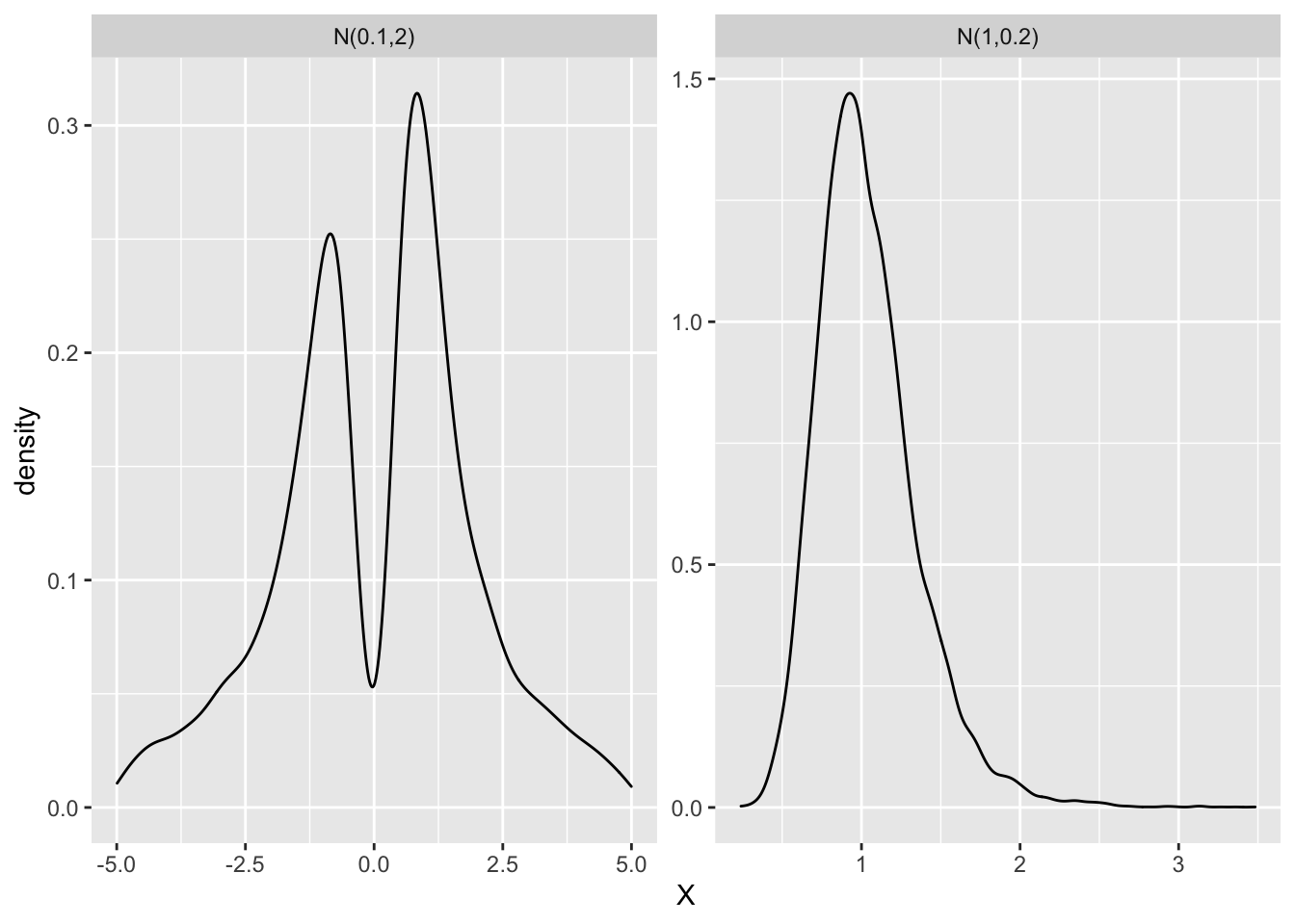
As the picture clearly shows, the ratio of two normals is no longer normal when the denominator has larger standard deviation with a mean closer to 0. It has two distinctive peaks and is bimodal.

Why is this realization important? Recall, what the denominator of \(\beta_{IV}\) represents. The denominator - \(z^Tx\) - represents the covariance of \(x\) with instrument \(z\). So, when the covariance between \(x\) with \(z\) is small, it would be similar to a distribution with large standard deviation and small mean. And we can see in the example above, that when that happens, the ratio of two normals is likely bimodal³. When the covariance between \(x\) with \(z\) is small, such an IV is refered to as a “weak IV”.

Weak IV and asymptotic approximation

The simple simulation above shows that weak IVs are problematic. But, the simulation approach isn’t reliable for estimating the uncertainty of \(\beta_{IV}\) for any IVs. For that one needs to finds an exact analytical expression of the sampling distribution of \(\beta_{IV}\). However, since the expression \(\frac{z^Ty}{z^Tx}\) is non-linear, it’s not possible to find an analytical expression. Then we rely on theoretical asymptotic methods to approximate the sampling distribution for larger samples. The standard errors of this theoretical asymptotic distribution would give us some sense of the uncertainty around the parameter. But, then the question is - does the finite sample distribution mirror the theoretical large sample approximation?

Using simulations, Rossi shows that the finite sampling distribution of \(\beta_{IV}\) can be different from its asymptotic approximation given by \((\frac{z^Tx}{N})^{-1} \sqrt N \frac{z^T \epsilon_y}{N}\). He compared the distribution of random variables coming from \(z^Ty/z^Tx\) versus distribution of normal random variables coming from \(\sqrt N \times z^T\epsilon_y\)⁴.

I demonstrate this by first choosing \(X_2 \sim N(0.1,1)\) as the denominator.

numerator <- rnorm(10e3,1,0.5)
denominator <- rnorm(10e3,0.1,1)
#Rossi mentions he trims 1% of the data
q_n <- quantile(numerator,c(0.01,0.99))
q_d <- quantile(denominator,c(0.01,0.99))
numerator_n <- numerator[numerator > q_n[1] & numerator < q_n[2]]
denominator_n <- denominator[denominator > q_d[1] & denominator < q_d[2]]
#asymptotic distribution
N <- length(numerator_n)
asymp_numerator_n <- sqrt(N)*(numerator_n)
 
data.frame(dist = numerator_n/denominator_n,
           # scale it down
           asymp_dist = asymp_numerator_n/100) %>%
  filter(dist > -20 & dist < 20) %>%
  ggplot() +
   geom_histogram(aes(x = dist, y = ..density..),binwidth = 0.3,color = "black") +
   geom_density(aes(x = asymp_dist), col = "green")

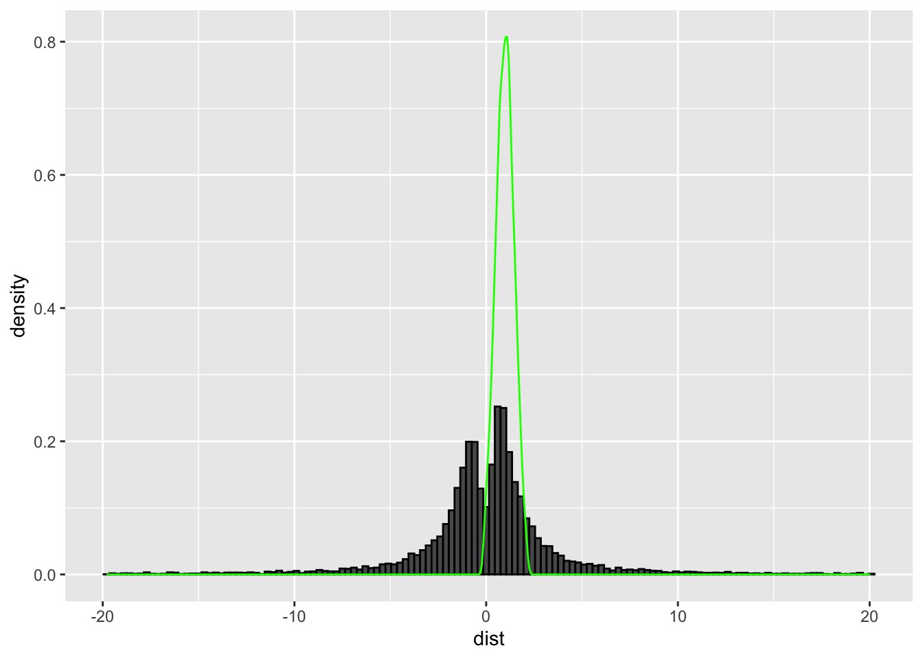
The asymptotic distribution in green does not come close to being similar in shape to the finite sample approximation which is bimodal. But if we were to perform the same test but this time by choosing \(X_2 \sim N(1,0.2)\) in the denominator -

numerator <- rnorm(10e3,1,0.5)
denominator <- rnorm(10e3,1,0.2)
q_n <- quantile(numerator,c(0.01,0.99))
q_d <- quantile(denominator,c(0.01,0.99))
numerator_n <- numerator[numerator > q_n[1] & numerator < q_n[2]]
denominator_n <- denominator[denominator > q_d[1] & denominator < q_d[2]]
N <- length(numerator_n)
asymp_numerator_n <- sqrt(N)*(numerator_n)
 
data.frame(dist = numerator_n/denominator_n,
           asymp_dist = asymp_numerator_n/100) %>%
  filter(dist > -20 & dist < 20) %>%
  ggplot() +
   geom_histogram(aes(x = dist, y = ..density..),binwidth = 0.3,color = "black") +
   geom_density(aes(x = asymp_dist), col = "green")

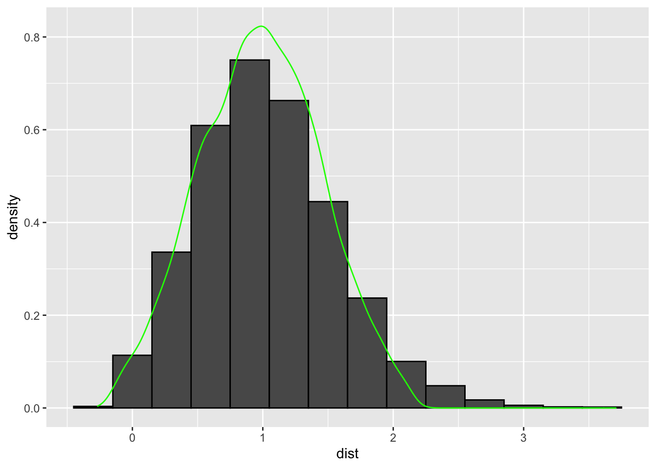
The asymptotic distribution in green does come close to being similar in shape to the finite sample approximation.

So, the lesson here is that asymptotic sampling theories, that help define the standard errors of IV estimates, are only valid when IVs are not weak. For weak IVs, Rossi points out that the asymptotic standard errors would be smaller compared to the actual standard errors which would then create issues for constructing correct confidence intervals.

We can use a statistical test to determine if an instrument is weak - if the first stage F stat is greater than 10, then the IV is not weak and the asymptotic approximation of sampling distribution is valid. Using instruments is then justified since it would help address the omitted variable bias in OLS estimates. Rossi demonstrates that this may not be true with another set of simulations. He simulates data from the following model -

$$y = -2x + \epsilon_y$$

Here \(y\) is the DV and \(x\) is the endogenous variable. There is an instrument \(z\) that related to \(x\) according to -

$$x = z\delta + \epsilon_x$$

Rossi chooses a modest population R-squared for this relationship equal to 0.1. So, the instrument is neither too strong nor too weak. Below, I generate data according to this specification. Then, I fit an OLS and IV model using this data to extract the coefficients on \(x\).

sim_IV <- function(){
  # covariance matrix on page 662
  cov_matrix <- matrix(c(1,0.25,0.25,1),byrow = T,nrow = 2)
  # errors from this covariance matrix
  error <- MASS::mvrnorm(n = 100,rep(0,2),cov_matrix)
  # z has a uniform distribution - page 662
  Z <- runif(100)
  # the relationship between x and z with delta = 1
  X <- Z + error[,1]
  # the relationship between y and x depicted above
  Y <- -2*X + error[,2]
  
  r_sq <- summary(lm(X ~ Z))$r.squared
  # OLS model
  ols <- lm(Y ~ X)
  # IV - 2SLS model
  f_stage <- lm(X ~ Z)
  pred_X <- predict(f_stage)
  s_stage <- lm(Y ~ pred_X)
  
  return(list(r_sq,
              coef(ols)['X'],
              coef(s_stage)['pred_X'],
              summary(f_stage)$fstatistic[1]))
}

I repeat the fitting process several times to generate histograms of the coefficient of \(x\) from the OLS and IV model.

all_simulations <- replicate(n = 2000,sim_IV())

Next, I extract the coefficient of \(x\) from the IV and OLS model from the repititions and plot them -

dt_coefs <-
  data.frame(ols_coeffs = unlist(all_simulations[2,]),
             iv_coeffs = unlist(all_simulations[3,])) %>%
  mutate(nsims = 1:n()) %>%
  tidyr::gather(key = type, value = coefficient, -nsims) %>%
  filter(coefficient < 1 & coefficient > -5) %>%
  mutate(type = as.factor(type),
         sq_err = round((coefficient + 2)^2,4))

ggplot(dt_coefs,aes(x = coefficient, y = ..density.., fill = type)) +
  geom_histogram(color = "black", binwidth = 0.03) +
  geom_vline(xintercept = -2, col = "blue", lty = 2) +
  theme(legend.position = "top") +
  scale_y_continuous(breaks = seq(0,10,1))

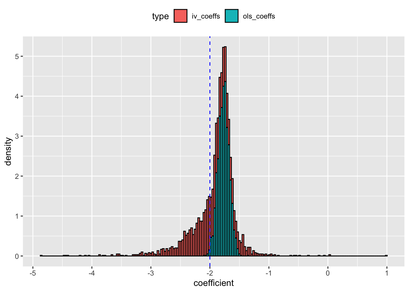
The blue line represents the actual coefficient on \(x\). At first glance, the IV model seems to approximate the coefficient better than OLS - the distribution of estimates is centered around the true value of -2. But, let’s check the RMSE on the coefficients from the two models.

dt_coefs %>%
  filter(type == "ols_coeffs") %>% pull(sq_err) %>%
  mean() %>% sqrt()

## [1] 0.2501555

dt_coefs %>%
  filter(type == "iv_coeffs") %>% pull(sq_err) %>%
  mean() %>% sqrt()

## [1] 0.449526

The RMSE from IV model is much higher than OLS. Even though the IV estimates are centered around actual value, it has thicker tails and it is more spread out leading to higher RMSE and poor sampling behavior. In comparison, the OLS estimates are more compact and has a lower RMSE. Next, I check the distribution of the first stage F values from all the simulations.

ggplot(data.frame(F_val = unlist(all_simulations[4,])),aes(x = F_val)) +
  geom_histogram(binwidth = 1, color = "black") +
  geom_vline(xintercept = 10, col = "blue", lty = 2) +
  labs(x = "F value")

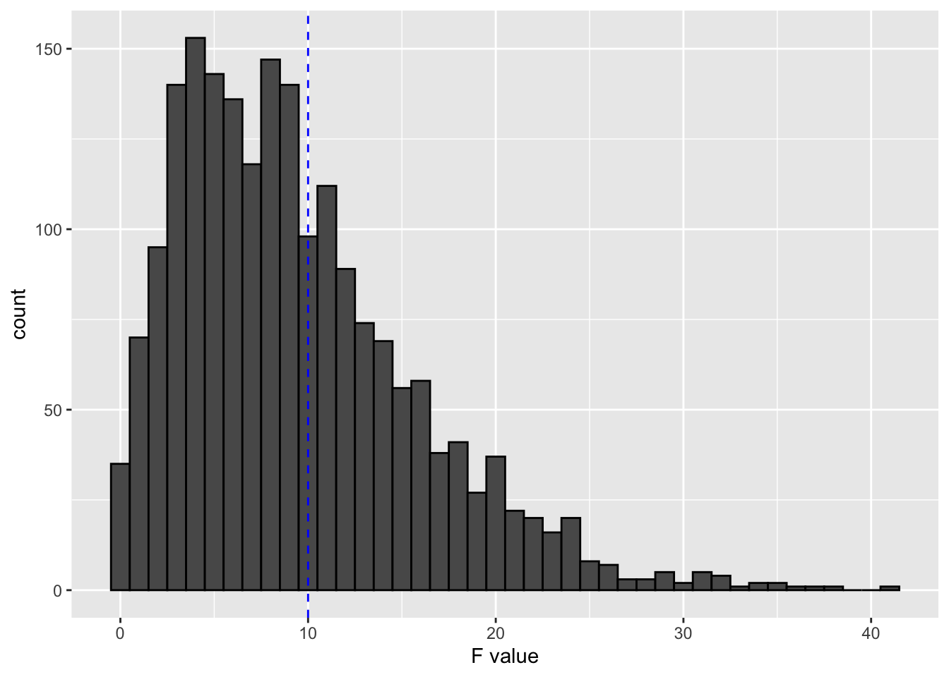
The graph shows that half of the simulations had F values that were above 10 for an instrument with population R-squared of 0.1. So, even though such an instrument could pass the weak IV check, it could end up creating a bigger RMSE (and poorer sampling behavior) compared to OLS.

Rossi also investigates if multiple weak IVs can alleviate the above concern. He simulates data using the same model as above. But this time he using 10 IVs. Althogether, these IVs have a population R squared value of 0.1 as before. Below I generate data by adjusting for the IV matrix and then fit an OLS and IV model. After that, I plot the estimates of \(x\) from the simulations from the OLS and IV model and report their MSEs.

sim_IV <- function(){
  cov_matrix <- matrix(c(1,0.25,0.25,1),byrow = T,nrow = 2)
  error <- MASS::mvrnorm(n = 100,rep(0,2),cov_matrix)
  Z <- matrix(replicate(10,runif(100)), ncol = 10)
  X <-  Z %*% matrix(rep(0.05,10)) + error[,1]
  Y <- -2*X + error[,2]
  r_sq <- summary(lm(X ~ Z))$r.squared
  ols <- lm(Y ~ X)
  f_stage <- lm(X ~ Z)
  pred_X <- predict(f_stage)
  s_stage <- lm(Y ~ pred_X)
  return(list(r_sq,coef(ols)['X'],coef(s_stage)['pred_X']))
}
all_simulations <- replicate(n = 2000,sim_IV())

dt_coefs <-
  data.frame(ols_coeffs = unlist(all_simulations[2,]),
             iv_coeffs = unlist(all_simulations[3,])) %>%
  mutate(nsims = 1:n()) %>%
  tidyr::gather(key = type, value = coefficient, -nsims) %>%
  mutate(type = as.factor(type),
         sq_err = round((coefficient + 2)^2,4))

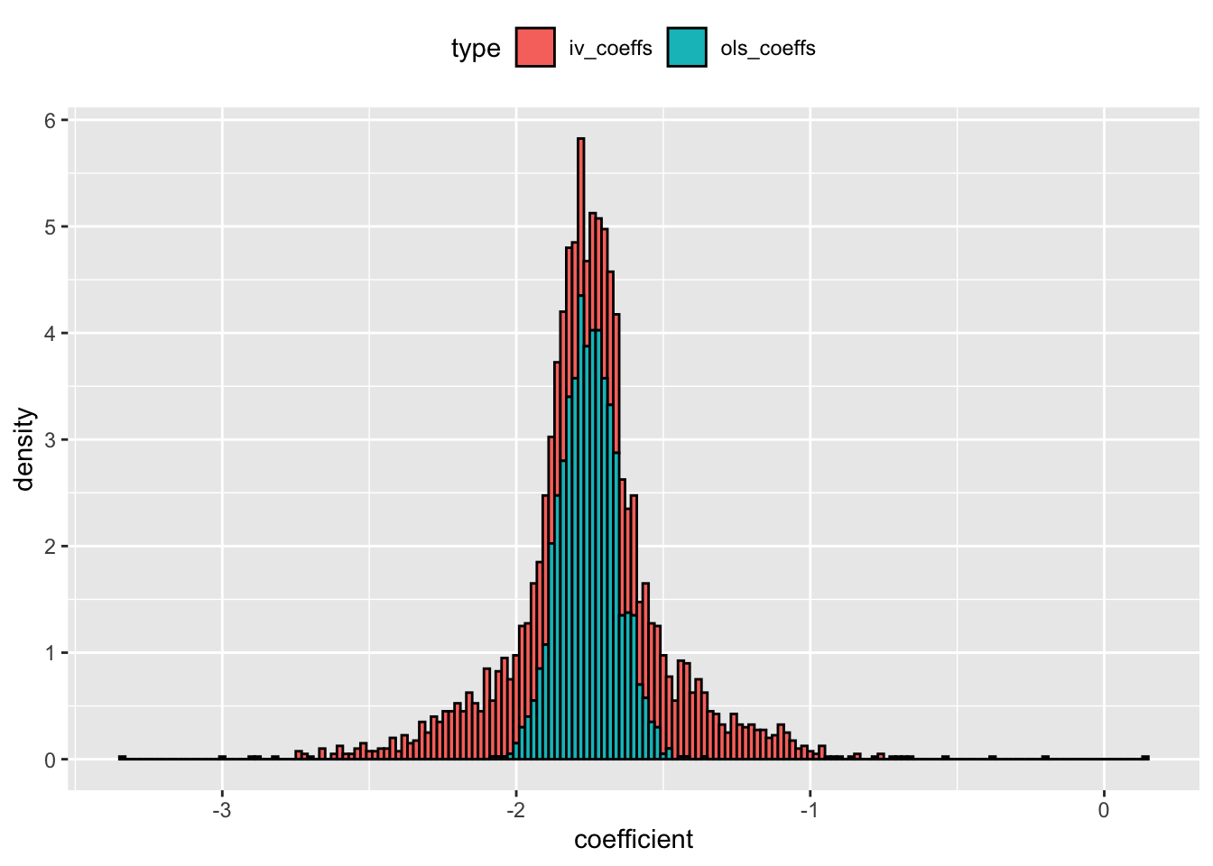
ggplot(dt_coefs,aes(x = coefficient,y = ..density.., fill = type)) +
  geom_histogram(color = "black", binwidth = 0.02) +
  theme(legend.position = "top") +
  scale_y_continuous(breaks = seq(0,10,1))

dt_coefs %>%
  filter(type == "ols_coeffs") %>% pull(sq_err) %>%
  mean() %>% sqrt()

## [1] 0.2635385

dt_coefs %>%
  filter(type == "iv_coeffs") %>% pull(sq_err) %>%
  mean() %>% sqrt()

## [1] 0.4233587

The results re-inforces the previous conclusion - multiple moderately weak IVs can still create as much RMSE as OLS estimates.

Is it valid though?

The results so far tell us that if the instruments are moderately strong, then (1) the estimates from small samples will be ‘normal’, (2) the large sample approximation of the estimate will be close to the small sample estimate and (3) the standard errors will be reliable.

But, Rossi points out that being moderately strong isn’t the only condition that makes IVs valid. For instruments to be valid, it should satisfy one more condition - the instrument must be uncorrelated with the error term⁵ \(\epsilon_y\). In other words, instrument \(z\) should only impact \(y\) through endogenous variable \(x\). Rossi uses another simulation to examine the reliability of \(\beta_{IV}\) when the IV is strong but invalid.

He simulates data from the following model -

$$y = -2x - z + \epsilon_y$$

Here \(y\) is the DV and \(x\) is the endogenous variable with \(z\) as an instrument of \(x\). Notice, \(z\) is related to \(\epsilon_y\) by construction which makes it invalid. To complete the model, he then relates \(z\) and \(x\) via -

$$x = 2z + \epsilon_x$$

As before, I generate data and then fit an OLS and IV model to extract the coefficients on \(x\).

# a function to simulate and return coefficients for x
sim_IV <- function(){
  # covariance matrix on page 661
  cov_matrix <- matrix(c(1,0.25,0.25,1),byrow = T,nrow = 2)
  # errors from this covariance matrix
  error <- MASS::mvrnorm(n = 500,rep(0,2),cov_matrix)
  # z has a uniform distribution - page 661
  Z <- runif(500)
  # create x using z and error_x
  X <- 2*Z + error[,2]
  # create y using x,z and error_y
  Y <- -2*X - Z + error[,1]
  # check to see if R-sq is close to 0.25 - page 661
  r_sq <- summary(lm(X ~ Z))$r.squared
  # OLS model of y and x
  ols <- lm(Y ~ X)
  # 2SLS IV model of y and x
  f_stage <- lm(X ~ Z)
  pred_X <- predict(f_stage)
  s_stage <- lm(Y ~ pred_X)
  # get the estimates of x from OLS and IV
  return(list(r_sq,
              coef(ols)['X'],
              coef(s_stage)['pred_X']))
}

I repeat the fitting process several times to generate histograms of the coefficient of \(x\) from the OLS and IV model.

set.seed(123)
all_simulations <- replicate(n = 2000,sim_IV())

# store it in a data set
dt_coefs <-
  data.frame(ols_coeffs = unlist(all_simulations[2,]),
             iv_coeffs = unlist(all_simulations[3,])) %>%
  mutate(nsims = 1:n()) %>%
  tidyr::gather(key = type, value = coefficient, -nsims) %>%
  mutate(type = as.factor(type),
         type2 = as.factor(ifelse(type == "iv_coeffs","IV","OLS")),
  # calculate MSE of the OLS and IV estimator
         sq_err = round((coefficient + 2)^2,4))

ggplot(dt_coefs,aes(x = coefficient, fill = type, y = ..density..)) +
  geom_histogram(color = "black", binwidth = 0.01) +
  geom_vline(xintercept = -2, col = "blue", lty = 2) +
  scale_y_continuous(breaks = seq(0,10,2)) +
  theme(legend.position = "top")

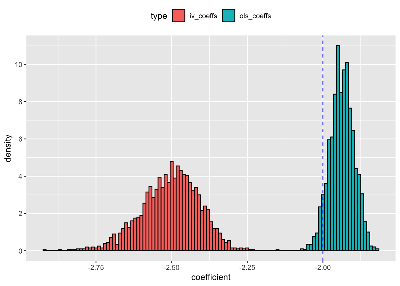
The blue line in the picture represents the true value of \(\beta\) on \(x\). The plot shows that both OLS and IV estimator are inaccurate because majority of the model estimates are either to the left (for the IV model) or on the right (on the OLS model) of true \(\beta\). The RMSE for IV estimator is equal to

dt_coefs %>%
  filter(type == "iv_coeffs") %>% pull(sq_err) %>%
  mean() %>% sqrt()

## [1] 0.5134721

And the RMSE for the OLS estimator is

dt_coefs %>%
  filter(type == "ols_coeffs") %>% pull(sq_err) %>%
  mean() %>% sqrt()

## [1] 0.07436868

The RMSE on IV estimate is almost 7 times the RMSE on the OLS estimate! So, even when the IV is not weak, its invalidity has made its sampling behavior worse than OLS.

But, what can we do to inspect whether the IV is invalid or not? Unfortunately, there are no statistical test, that can help us inspect whether an IV is invalid⁶. In the end, Rossi argues that because, we can never objectively test for IV validity, the idea that IV models should be preferred over OLS models “is not persuasive”.